This post presents a detailed walkthrough of a solution to
Standford CS231n:Convolutional Neural Networks for Visual Recognition course (Spring 2025).
This post is not only to provide working solution code, but to explain the underlying concepts, step by step,
so you can build a deeper unerstanding of how and why the solution works.
You can find the complete solution code on my github repo → click this link.
This post is just about the hard part of the assignment. And please keep in mind that some parts of solution may not be fully correct or understanable. If you spot any mistakes or areas for improvement, feel free to let me know. I'd truly appreciate it.
This post is just about the hard part of the assignment. And please keep in mind that some parts of solution may not be fully correct or understanable. If you spot any mistakes or areas for improvement, feel free to let me know. I'd truly appreciate it.
Index
- Q1:k-Nearest Neighbor classifier
- Q2:Implement a Softmax Classifier
- Q3:Two-Layer Neural Network
- Q4: Higher Level Representations: Image Features (__skip__)
- Q5: Training a fully connected network (__skip__)
- Q1: Batch Normalization
- Q2: Dropout (__skip__)
- Q3: Convolutional Neural Networks
- Q4: PyTorch on CIFAR-10 (__skip__)
- Q5: Image Captioning with Vanilla RNNs (__skip__)
Assignment1
Q1:k-Nearest Neighbor classifier
Implementing no-loop
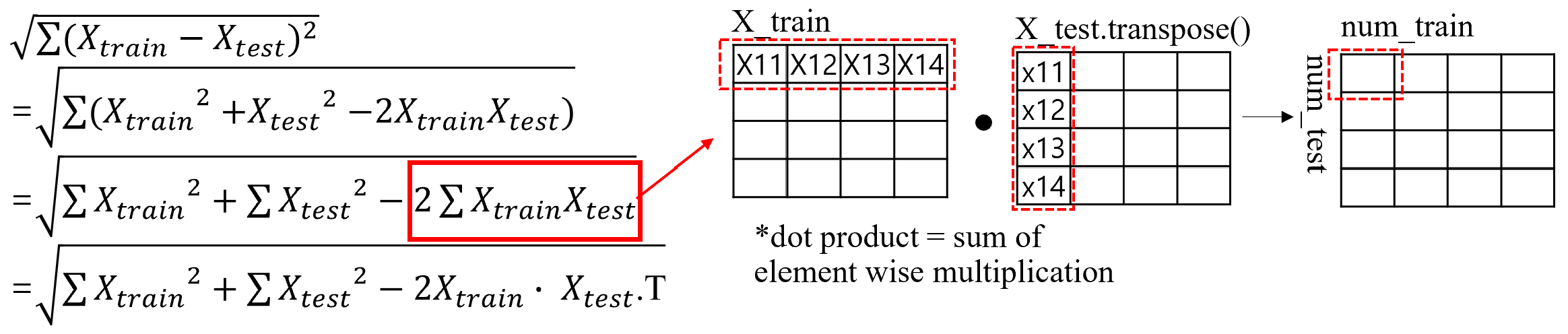 To approach the most challenging no-loop implementation, we start by expanding the quadratic equation used in the the K-Nearest Neighbors (KNN) algorithm.
The self-squared terms can be simply computed using
To approach the most challenging no-loop implementation, we start by expanding the quadratic equation used in the the K-Nearest Neighbors (KNN) algorithm.
The self-squared terms can be simply computed using np.sum() and np.square().
For cross term, since it involves the sum of element-wise multiplications, it can be converted to a dot product.
However, be careful to transpose one of the matrices to match alignment (see picture below).
Q2:Implement a Softmax Classifier
Numeric stability
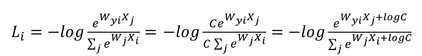
The exponentiating each score using the natural constant lead to large values and incur numeric instability. To address this issue, subtract the maximum score across all scores. This operation doesn't affect loss function because dividing both numerator and denominator by the same value leaves the result unchanged. Addtionally, should add a very small epsilon after subtracting to avoid taking logarithm of zero.
Computing gradient
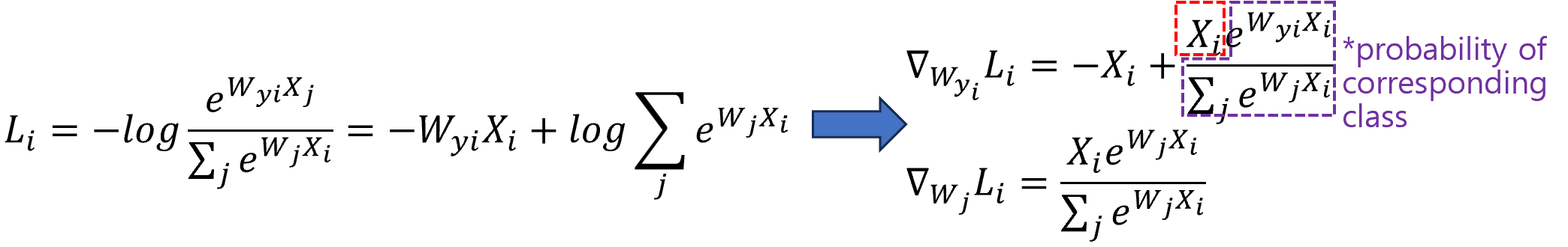 Take the derivatives with respect to the weights of the correct class label and the other class separately.
For both weights, the gradient invloves multiplication of input data and the corresponding class probability.
However, for the correct class label, the gradient gets subtracted by input data. Let's walk through a simple example, where we use softmax to train 1x3 input vector for 3-class classification task.
Take the derivatives with respect to the weights of the correct class label and the other class separately.
For both weights, the gradient invloves multiplication of input data and the corresponding class probability.
However, for the correct class label, the gradient gets subtracted by input data. Let's walk through a simple example, where we use softmax to train 1x3 input vector for 3-class classification task.
          X = [3.0, -2.6, 2.0]
          W = np.random([3,3])
          prb = [0.2, 0.6, 0.1]
          Y = [1,0,0]

          dW[0] = -X + X*0.2
          dW[1] = X*0.6
          dW[0] = X*0.1
Implementing no-loop gradient
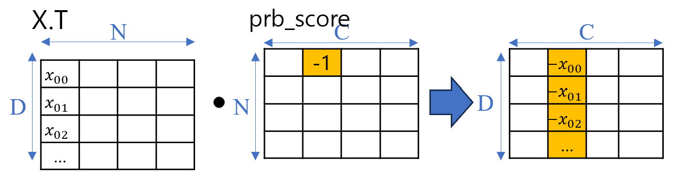
We can implement multiplication between input data and corresponding probability with simple dot product between input batch data and the probability matrix. This matrix contains the predicted probability scores for each class across all samples. To implement subtraction for correct class in the gradient, we need to slightly modify the probability matrix. Specifically, we subtract
1 at the position of corresponding to correct class bel for each sample.
As shown in picture abov,e if the correct label for the first sample is class 2, then -1 is added (not replaced) at the position in the matrix.
Q3:Two-Layer Neural Network
Computing gradient
The best way to understand fully-connected layer is writing down all computations manually. Let's walk through a simple example where 2x3 input vector and 3x2 weight vector. Assume2x2 dout comes from the upstream layer in the network.
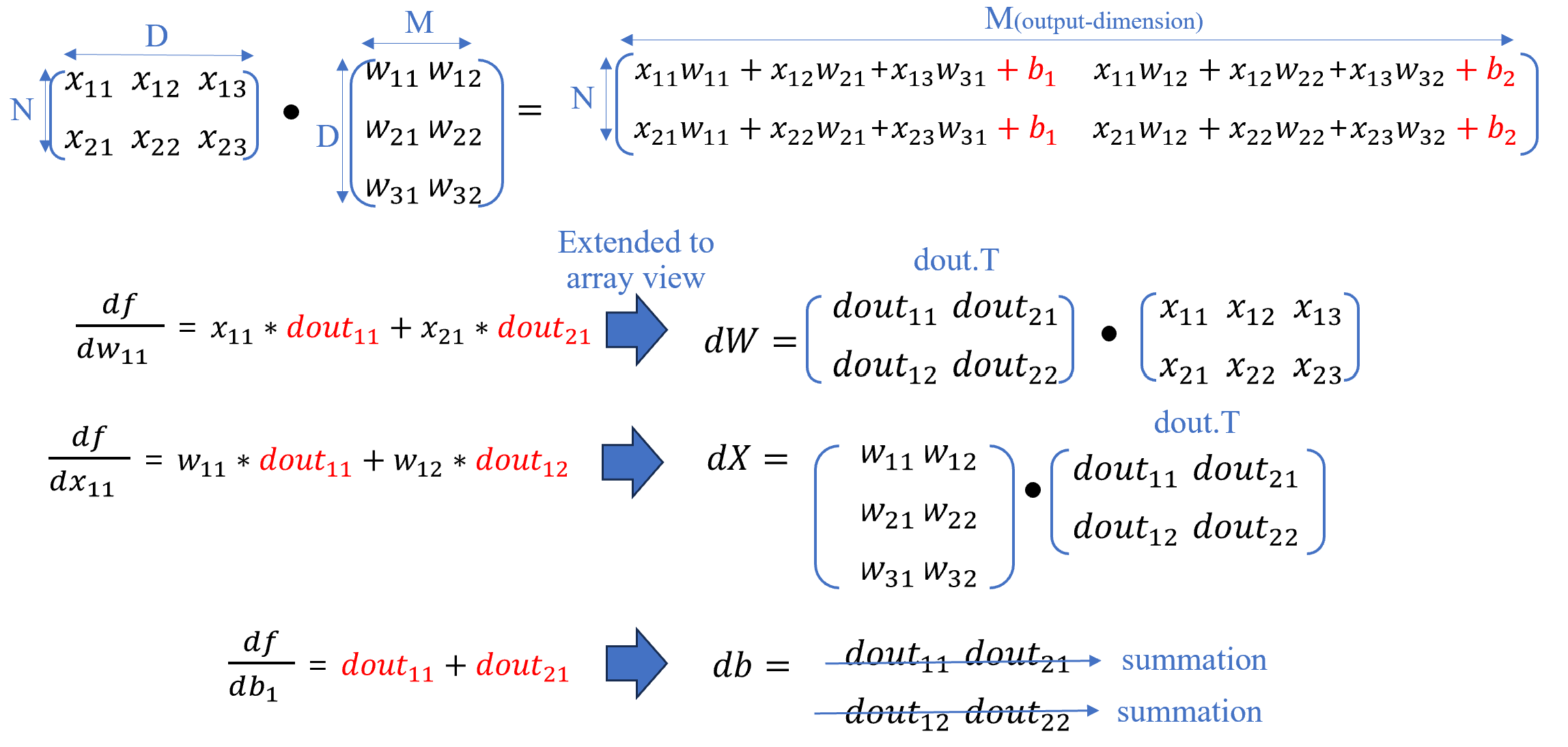 As seen above picture, the gradient of weight and input are another dot product and that of bias is simple summation along axis.
The remaining part mainly involves assembling the components and just setting up the training loop, which are relatively straightforward, so I'll skip over them here.
Assignment2
Q1: Batch Normalization
Getting gradient of gamma and beta
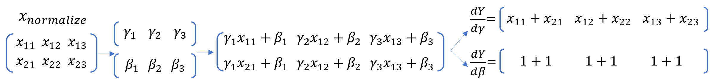 The gradient beta and gamma are simply calculated by summing over the appropriate axis.
You can refer to the illustration above using 2x3 input vector.
The gradient beta and gamma are simply calculated by summing over the appropriate axis.
You can refer to the illustration above using 2x3 input vector.
Getting gradient of input
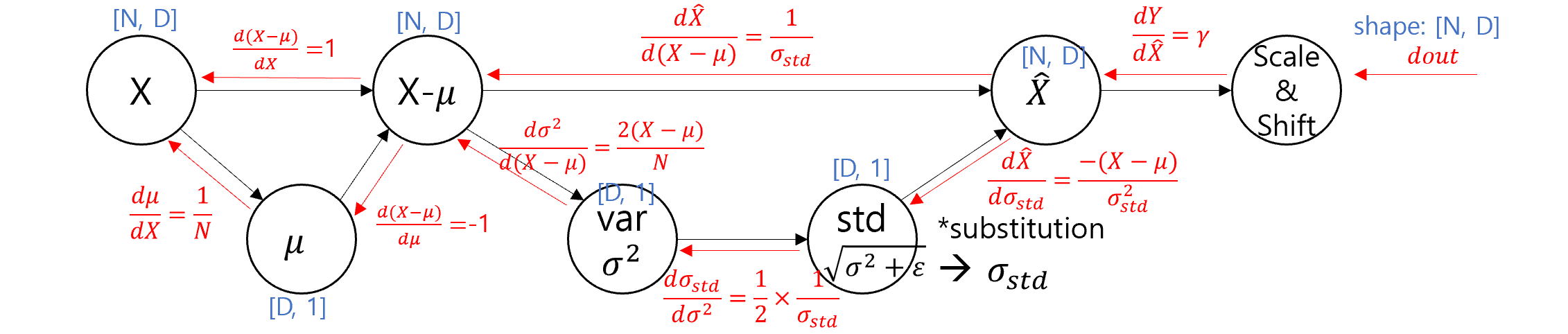 We need to backpropagate through the entire computational graph.
This invloves tracing the full path backward-from the final output, through the normalization step, and back to the original input-while applying the chain rule at each stage.
Please take care to apply proper reshaping, as it is essential to align gradient correctly.
For example, when tracing the path from the normalized input (shape [N,D]) to the standard deviation (shape [D,1]), you'll need to reduce the dimension by summing over the axis.
We need to backpropagate through the entire computational graph.
This invloves tracing the full path backward-from the final output, through the normalization step, and back to the original input-while applying the chain rule at each stage.
Please take care to apply proper reshaping, as it is essential to align gradient correctly.
For example, when tracing the path from the normalized input (shape [N,D]) to the standard deviation (shape [D,1]), you'll need to reduce the dimension by summing over the axis.
Q3:Convolutional Neural Networks
im2col (Image to Column)
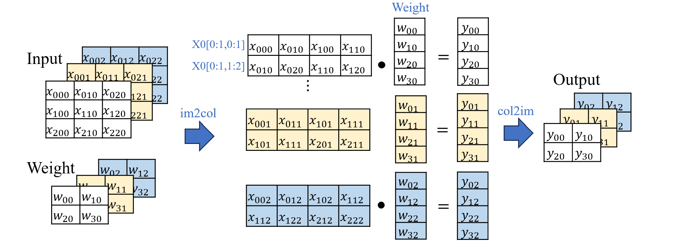 We will avoid using explicit loops to implement the sliding of the filter.
Instead, we use the im2col tenchnique, which transforms the input vector into a matrix which each row corresponds to a receptive field aligned with the filter's sliding window.
While this approach can lead to wastful memory footage-due to duplication-it can significantly accelerate computation by enabling efficient matrix multiplication.
Refer to the illustration above, which shows a convolution operation on a 3x3 input with 2x2 filter and stride 1.
We will avoid using explicit loops to implement the sliding of the filter.
Instead, we use the im2col tenchnique, which transforms the input vector into a matrix which each row corresponds to a receptive field aligned with the filter's sliding window.
While this approach can lead to wastful memory footage-due to duplication-it can significantly accelerate computation by enabling efficient matrix multiplication.
Refer to the illustration above, which shows a convolution operation on a 3x3 input with 2x2 filter and stride 1.
Getting gradient dW
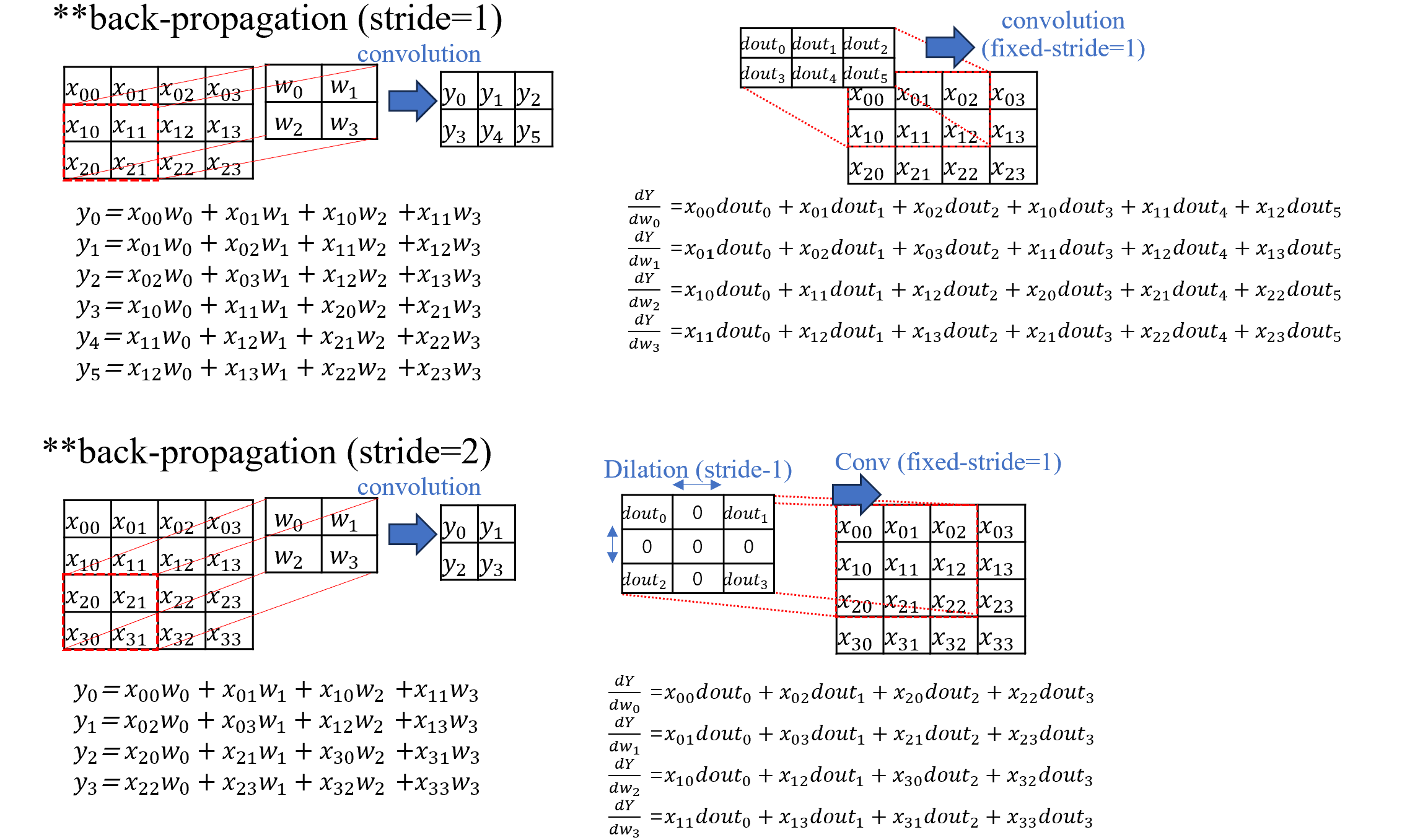 The gradient with respect to W is computed by convolving the input vector with tge gradient received from the upstrea layer.
The upstream gradient acts as the filter, and the stride is fixed to be 1.
When it comes to original stride of CNN, that is reflected during the backpropagation by dilating the upstream gradient.
Refering to stride-2 case in the illustration above will be helpful to understand.
The gradient with respect to W is computed by convolving the input vector with tge gradient received from the upstrea layer.
The upstream gradient acts as the filter, and the stride is fixed to be 1.
When it comes to original stride of CNN, that is reflected during the backpropagation by dilating the upstream gradient.
Refering to stride-2 case in the illustration above will be helpful to understand.
Getting gradient dX

The gradient with respect to input X is similiar excep that the weight acts as filter and dilation is applied to upstream gradient. Addtionally an extra one-pixel zero-padding is added around the upstream gradient. The illustration above demonstrates how to compute dX for a stride 2 case with 2x2 weight filter. Note that the resulting dX will include regions corresponding to the added zero-padding. These padded area are not part of the original input and must be explicitly trimmed to be the correct gradient.
Assignment2
Q1: Batch Normalization
Getting gradient of gamma and beta
The gradient beta and gamma are simply calculated by summing over the appropriate axis.
You can refer to the illustration above using 2x3 input vector.
Getting gradient of input
We need to backpropagate through the entire computational graph.
This invloves tracing the full path backward-from the final output, through the normalization step, and back to the original input-while applying the chain rule at each stage.
Please take care to apply proper reshaping, as it is essential to align gradient correctly.
For example, when tracing the path from the normalized input (shape [N,D]) to the standard deviation (shape [D,1]), you'll need to reduce the dimension by summing over the axis.
Q3:Convolutional Neural Networks
im2col (Image to Column)
We will avoid using explicit loops to implement the sliding of the filter.
Instead, we use the im2col tenchnique, which transforms the input vector into a matrix which each row corresponds to a receptive field aligned with the filter's sliding window.
While this approach can lead to wastful memory footage-due to duplication-it can significantly accelerate computation by enabling efficient matrix multiplication.
Refer to the illustration above, which shows a convolution operation on a 3x3 input with 2x2 filter and stride 1.
Getting gradient dW
The gradient with respect to W is computed by convolving the input vector with tge gradient received from the upstrea layer.
The upstream gradient acts as the filter, and the stride is fixed to be 1.
When it comes to original stride of CNN, that is reflected during the backpropagation by dilating the upstream gradient.
Refering to stride-2 case in the illustration above will be helpful to understand.
Getting gradient dX
The gradient with respect to input X is similiar excep that the weight acts as filter and dilation is applied to upstream gradient. Addtionally an extra one-pixel zero-padding is added around the upstream gradient. The illustration above demonstrates how to compute dX for a stride 2 case with 2x2 weight filter. Note that the resulting dX will include regions corresponding to the added zero-padding. These padded area are not part of the original input and must be explicitly trimmed to be the correct gradient.
Assignment3
Q1:Image Captioning with Transformers
Implementing Multihed Self-Attention Layer
Q2:Self-Supervised Learning for Image Classification
Implementing vectorized SimCLR loss
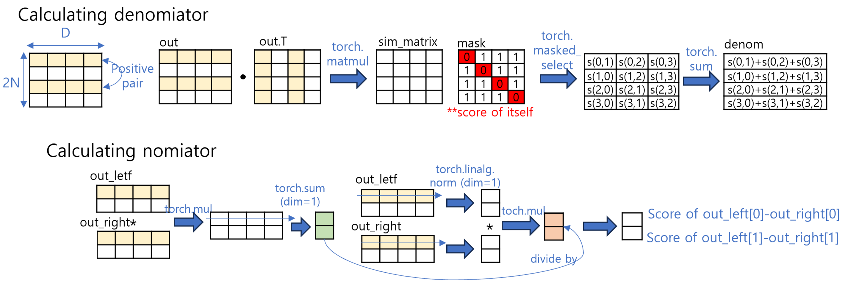 SimCLR expands each batch from [N,D] to [2N,D] using two augmentations per image.
The yellow box indicates one of positive pair.
In vectorized form, cosine similarity can be efficiently computed using simple matrix multiplication for denominator of loss and element-wise multiplcation for nomnator.
However, don't forget to mask-out in denominator for InfoNCE which exclude score of itself.
SimCLR expands each batch from [N,D] to [2N,D] using two augmentations per image.
The yellow box indicates one of positive pair.
In vectorized form, cosine similarity can be efficiently computed using simple matrix multiplication for denominator of loss and element-wise multiplcation for nomnator.
However, don't forget to mask-out in denominator for InfoNCE which exclude score of itself.