- Replace explicit Python loops in KNN and Softmax classifiers with matrix expansion and in-place probability matrix adjustments for orders-of-magnitude faster execution.
- Derive Batch Normalization and Spatial Batch/Group Normalization backward gradients systematically by decomposing the computational graph into intermediate partial derivatives.
- Accelerate 2D convolutions and their backward passes (dW, dX) via im2col receptive-field matrix unrolling and dilated upstream gradients for strided convolutions.
- Implement batched Multi-Head Self-Attention, vectorized SimCLR InfoNCE contrastive loss, and closed-form DDPM forward/reverse sampling steps.
This post presents a detailed walkthrough of a solution to Standford CS231n:Convolutional Neural Networks for Visual Recognition course (Spring 2025). This post is not only to provide working solution code, but to explain the underlying concepts, step by step, so you can build a deeper unerstanding of how and why the solution works.
This post is just about the hard part of the assignment. And please keep in mind that some parts of solution may not be fully correct or understanable. If you spot any mistakes or areas for improvement, feel free to let me know. I’d truly appreciate it.
Assignment1
Q1: KNN - implementing no loop
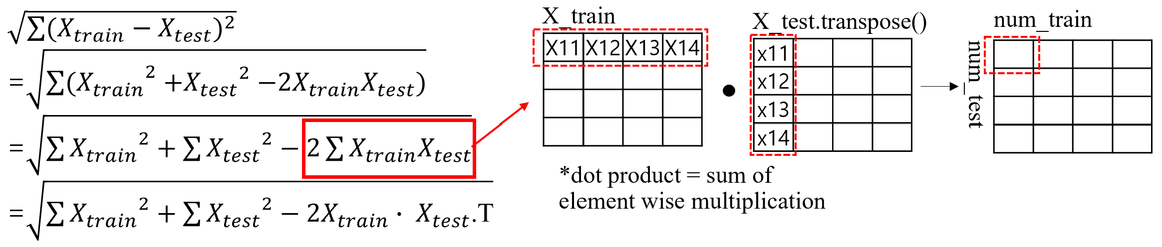
To approach the most challenging no-loop implementation, we start by expanding the quadratic equation used in the the K-Nearest Neighbors (KNN) algorithm. The self-squared terms can be simply computed using np.sum() and np.square(). For cross term, since it involves the sum of element-wise multiplications, it can be converted to a dot product. However, be careful to transpose one of the matrices to match alignment.
def compute_distances_no_loops(self, X):
    """
    Compute the distance between each test point in X and each training point
    in self.X_train using no explicit loops.
    Input / Output: Same as compute_distances_two_loops
    """
    num_test = X.shape[0]
    num_train = self.X_train.shape[0]
    dists = np.zeros((num_test, num_train))

    X_train_sqr_sum = np.power(self.X_train, 2).sum(axis=1) # [5000,]
    X_test_sqr_sum = np.power(X, 2).sum(axis=1) # [500,]
    X_train_sqr_sum = np.repeat(X_train_sqr_sum, num_test)
    X_train_sqr_sum = X_train_sqr_sum.reshape(num_train, num_test) # [5000, 500]
    X_test_sqr_sum = np.repeat(X_test_sqr_sum, num_train)

    X_test_sqr_sum = X_test_sqr_sum.reshape(num_test, num_train) # [500, 5000]
    dists = np.sqrt(X_train_sqr_sum.T + X_test_sqr_sum - 2*X.dot(self.X_train.T))
    return dists
Q2:Implement a Softmax Classifier
Numeric stability

The exponentiating each score using the natural constant lead to large values and incur numeric instability. To address this issue, subtract the maximum score across all scores. This operation doesn’t affect loss function because dividing both numerator and denominator by the same value leaves the result unchanged. Addtionally, should add a very small epsilon after subtracting to avoid taking logarithm of zero.
Computing gradient

Take the derivatives with respect to the weights of the correct class label and the other class separately. For both weights, the gradient invloves multiplication of input data and the corresponding class probability. However, for the correct class label, the gradient gets subtracted by input data. Let’s walk through a simple example, where we use softmax to train 1x3 input vector for 3-class classification task.
X = [3.0, -2.6, 2.0]
W = np.random([3,3])
prb = [0.2, 0.6, 0.1]
Y = [1,0,0]

dW[0] = -X + X*0.2
dW[1] = X*0.6
dW[0] = X*0.1
Implementing no-loop gradient
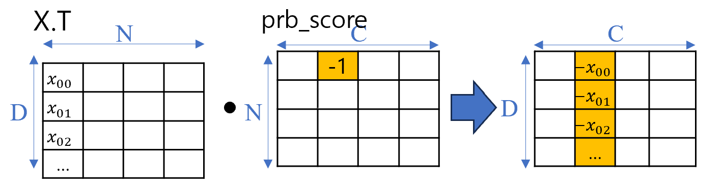
We can implement multiplication between input data and corresponding probability with simple dot product between input batch data and the probability matrix. This matrix contains the predicted probability scores for each class across all samples. To implement subtraction for correct class in the gradient, we need to slightly modify the probability matrix. Specifically, we subtract 1 at the position of corresponding to correct class bel for each sample. As shown in picture abov,e if the correct label for the first sample is class 2, then -1 is added (not replaced) at the position in the matrix.
The final code is:
def softmax_loss_vectorized(W, X, y, reg):
    """
    Softmax loss function, vectorized version.

    Inputs and outputs are the same as softmax_loss_naive.
    """
    # Initialize the loss and gradient to zero.
    loss = 0.0
    dW = np.zeros_like(W)


#############################################################################
    # TODO:                                                                     #
    # Implement a vectorized version of the softmax loss, storing the           #
    # result in loss.                                                           #
    #############################################################################
    num_train = X.shape[0]

    score = X.dot(W)
    score -= score.max(axis=1, keepdims=True)
    score += 1e-12 # to avoid log(0)
    score = np.exp(score)
    prb_score = score/score.sum(axis=1, keepdims=True) # numeric stability
    loss = -np.log(prb_score[np.arange(num_train),y]).sum()
    prb_score[range(num_train),y] -= 1

    loss /= num_train
    loss += reg * np.sum(W*W)
    #############################################################################
    # TODO:                                                                     #
    # Implement a vectorized version of the gradient for the softmax            #
    # loss, storing the result in dW.                                           #
    #                                                                           #
    # Hint: Instead of computing the gradient from scratch, it may be easier    #
    # to reuse some of the intermediate values that you used to compute the     #
    # loss.                                                                     #
    #############################################################################

    dW += X.T.dot(prb_score)
    dW /= num_train
    dW += 2 * reg * W

    return loss, dW
Q3: Two-Layer Neural Network, computing gradient
The best way to understand fully-connected layer is writing down all computations manually. Let’s walk through a simple example where 2x3 input vector and 3x2 weight vector. Assume 2x2 dout comes from the upstream layer in the network.
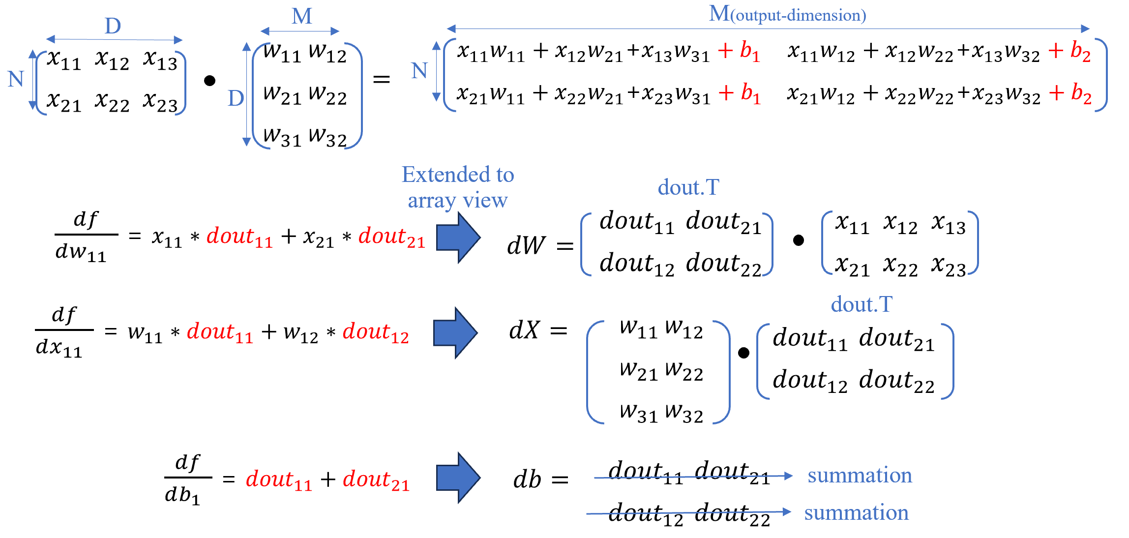
As seen above picture, the gradient of weight and input are another dot product and that of bias is simple summation along axis.
The remaining part mainly involves assembling the components and just setting up the training loop, which are relatively straightforward, so I’ll skip over them here
def affine_backward(dout, cache):
    """
    Computes the backward pass for an affine layer.

    Inputs:
    - dout: Upstream derivative, of shape (N, M)
    - cache: Tuple of:
      - x: Input data, of shape (N, d_1, ... d_k)
      - w: Weights, of shape (D, M)
      - b: Biases, of shape (M,)

    Returns a tuple of:
    - dx: Gradient with respect to x, of shape (N, d1, ..., d_k)
    - dw: Gradient with respect to w, of shape (D, M)
    - db: Gradient with respect to b, of shape (M,)
    """
    x, w, b = cache
    dx, dw, db = None, None, None
    ###########################################################################
    # TODO: Implement the affine backward pass.                               #
###########################################################################

    dx = w.dot(dout.T).T.reshape(x.shape)
    x_resh = x.reshape(x.shape[0], -1)
    dw = dout.T.dot(x_resh).T
    db = dout.sum(axis=0)

    return dx, dw, db
Assignment2
Q1: Batch Normalization
Getting gradient of gamma and beta

The gradient beta and gamma are simply calculated by summing over the appropriate axis. You can refer to the illustration above using 2x3 input vector.
Getting gradient of input
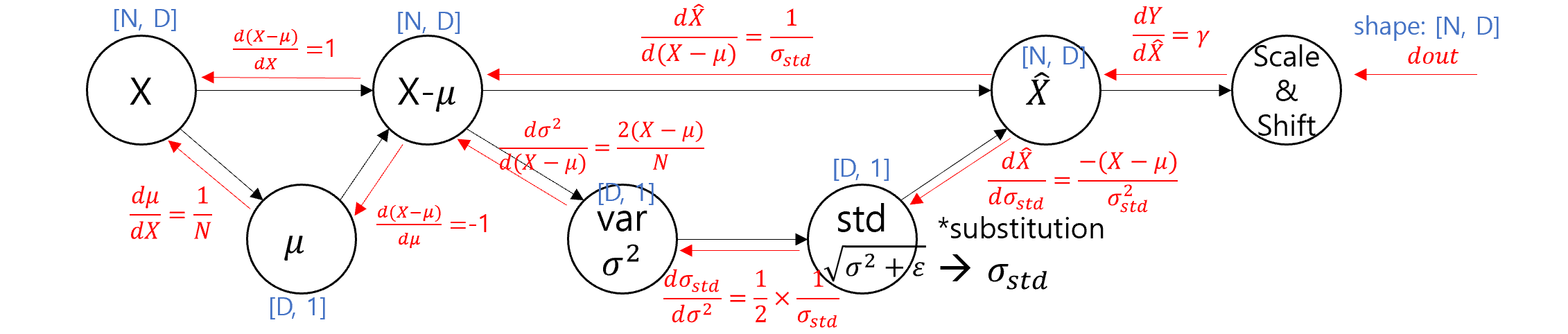
We need to backpropagate through the entire computational graph. This invloves tracing the full path backward-from the final output, through the normalization step, and back to the original input-while applying the chain rule at each stage. Please take care to apply proper reshaping, as it is essential to align gradient correctly. For example, when tracing the path from the normalized input (shape [N,D]) to the standard deviation (shape [D,1]), you’ll need to reduce the dimension by summing over the axis.
def batchnorm_backward(dout, cache):
    """Backward pass for batch normalization.

    For this implementation, you should write out a computation graph for
    batch normalization on paper and propagate gradients backward through
    intermediate nodes.

    Inputs:
    - dout: Upstream derivatives, of shape (N, D)
    - cache: Variable of intermediates from batchnorm_forward.

    Returns a tuple of:
    - dx: Gradient with respect to inputs x, of shape (N, D)
    - dgamma: Gradient with respect to scale parameter gamma, of shape (D,)
    - dbeta: Gradient with respect to shift parameter beta, of shape (D,)
    """
    dx, dgamma, dbeta = None, None, None
    ###########################################################################
    # TODO: Implement the backward pass for batch normalization. Store the    #
    # results in the dx, dgamma, and dbeta variables.                         #
    # Referencing the original paper (https://arxiv.org/abs/1502.03167)       #
    # might prove to be helpful.                                              #
    ###########################################################################
    x, x_norm, gamma, var, mu, eps = cache
    N = dout.shape[0]
    std = np.sqrt(var + eps)

    # easist one
    dgamma = np.sum(x_norm*dout, axis=0)
    dbeta = dout.sum(axis=0)

    # (core-part) dx

    dL_dxnorm = dout*gamma

    dL_dstd = np.sum(dL_dxnorm * -(x-mu), axis=0)/(std**2)
    dL_dvar = dL_dstd*0.5/std
    dL_dx_1 = dL_dxnorm/std + dL_dvar * 2*(x-mu) / N
    dL_dmu = -np.sum(dL_dx_1, axis=0)
    dL_dx_2 = dL_dmu / N

    dx = dL_dx_1 + dL_dx_2
    ###########################################################################
    #                             END OF YOUR CODE                            #
    ###########################################################################

    return dx, dgamma, dbeta
Q3: Convolutional Neural Networks
im2col (Image to Column)
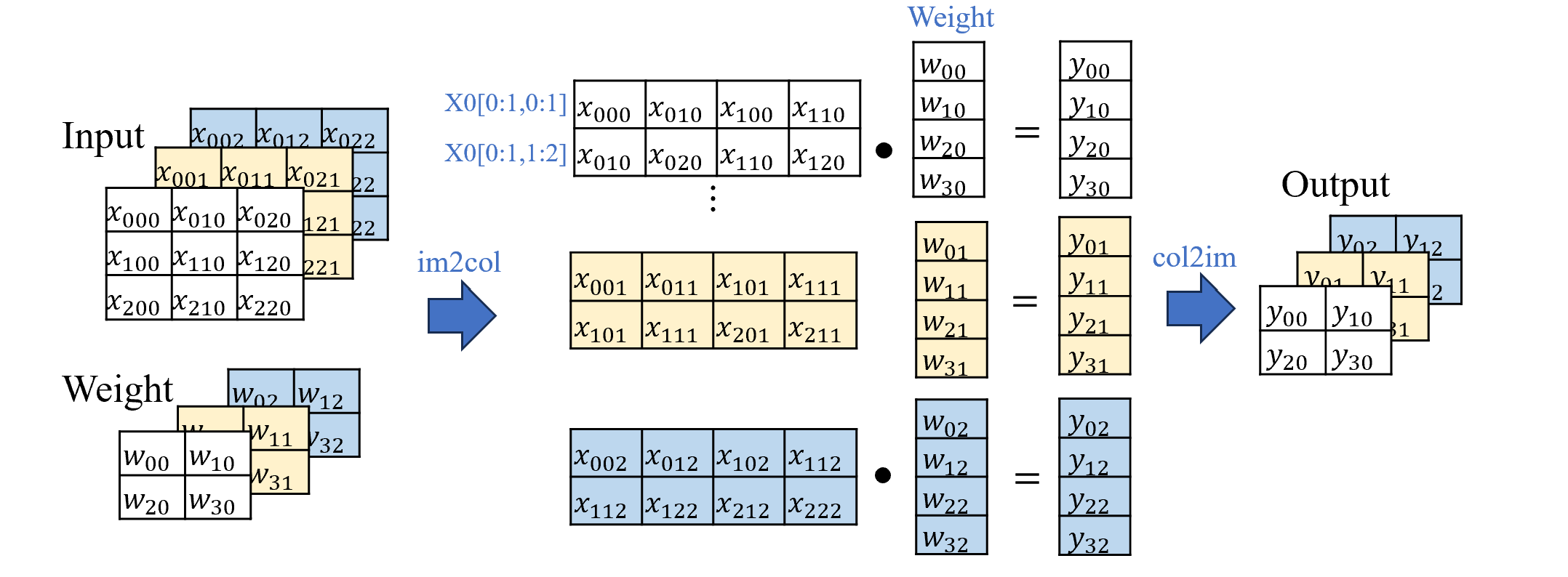
We will avoid using explicit loops to implement the sliding of the filter. Instead, we use the im2col tenchnique, which transforms the input vector into a matrix which each row corresponds to a receptive field aligned with the filter’s sliding window. While this approach can lead to wastful memory footage-due to duplication-it can significantly accelerate computation by enabling efficient matrix multiplication. Refer to the illustration above, which shows a convolution operation on a 3x3 input with 2x2 filter and stride 1.
def conv_forward_naive(x, w, b, conv_param):
    ....
    ###########################################################################
    # TODO: Implement the convolutional forward pass.                         #
    # Hint: you can use the function np.pad for padding.                      #
    ###########################################################################
    pad     = conv_param['pad']
    stride  = conv_param['stride']
    pad_dim = [(0,0), (0,0)] + [(pad, pad)] * 2

    x_pad = np.pad(x, pad_dim, mode='constant', constant_values=0)

    N, C, H, W = x_pad.shape
    F, CC, HH, WW = w.shape
    assert(C==CC)

    Hout = (H-HH)//stride+1
    Wout = (W-WW)//stride+1

    h_idx_s = np.arange(start=0, stop=H-HH+1, step=stride)
    h_idx_e = np.arange(start=HH, stop=H+1, step=stride)
    w_idx_s = np.arange(start=0, stop=W-WW+1, step=stride)
    w_idx_e = np.arange(start=WW, stop=W+1, step=stride)

    n_stride_w = len(w_idx_s)
    n_stride_h = len(h_idx_s)

    # x_pad im2col
    x_pad_im2col = np.zeros([N, Hout*Wout, HH*WW*C])
    for r in range(n_stride_h):
        for c in range(n_stride_w):
            x_pad_im2col[:,r*n_stride_w+c,:] = \
              x_pad[:,:,h_idx_s[r]:h_idx_e[r], w_idx_s[c]:w_idx_e[c]].reshape([N,HH*WW*C])

    # filter im2col
    w_im2col = w.reshape([F,HH*WW*C])
    conv_out = x_pad_im2col.dot(w_im2col.T) #[N, Hout*Wout, F]
    conv_out_swap = np.swapaxes(conv_out, 1, 2)

    out = conv_out_swap + b.reshape([1,F,1])
    out = out.reshape([N, F, Hout, Wout])

    ###########################################################################
    #                             END OF YOUR CODE                            #
    ###########################################################################
    cache = (x, w, b, conv_param)
    return out, cache
Getting gradient dW
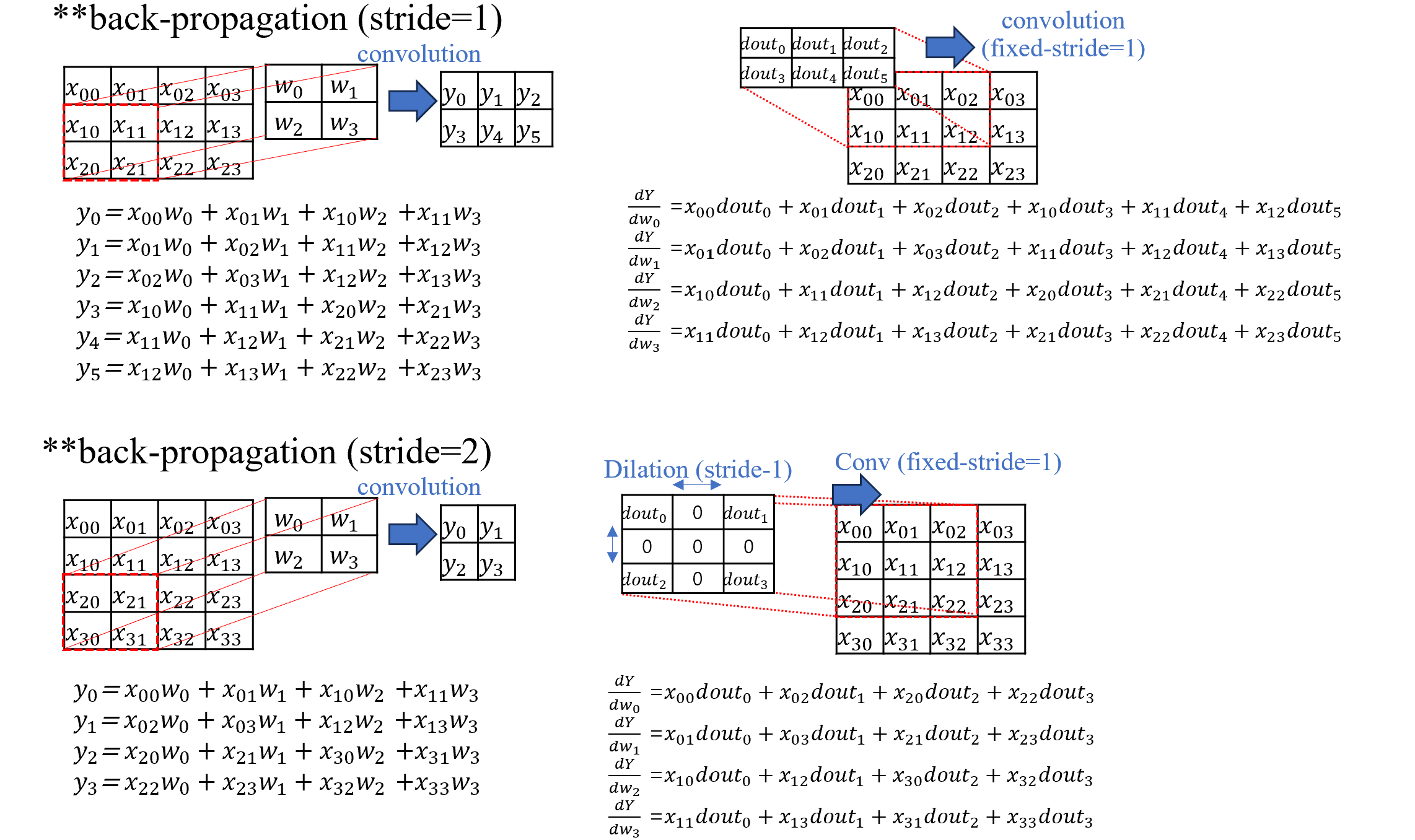
The gradient with respect to W is computed by convolving the input vector with tge gradient received from the upstrea layer. The upstream gradient acts as the filter, and the stride is fixed to be 1. When it comes to original stride of CNN, that is reflected during the backpropagation by dilating the upstream gradient. Refering to stride-2 case in the illustration above will be helpful to understand.
Getting gradient dX
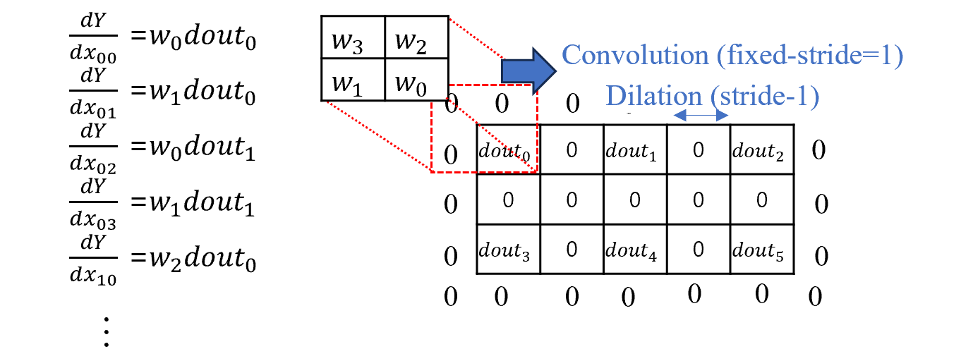
The gradient with respect to input X is similiar excep that the weight acts as filter and dilation is applied to upstream gradient. Addtionally an extra one-pixel zero-padding is added around the upstream gradient. The illustration above demonstrates how to compute dX for a stride 2 case with 2x2 weight filter. Note that the resulting dX will include regions corresponding to the added zero-padding. These padded area are not part of the original input and must be explicitly trimmed to be the correct gradient.
The final code:
def conv_backward_naive(dout, cache):
    """A naive implementation of the backward pass for a convolutional layer.

    Inputs:
    - dout: Upstream derivatives.
    - cache: A tuple of (x, w, b, conv_param) as in conv_forward_naive

    Returns a tuple of:
    - dx: Gradient with respect to x
    - dw: Gradient with respect to w
    - db: Gradient with respect to b
    """
    dx, dw, db = None, None, None
    ###########################################################################
    # TODO: Implement the convolutional backward pass.                        #
    ###########################################################################
    x, w, b, conv_param = cache

    pad     = conv_param['pad']
    stride  = conv_param['stride']
    pad_dim = [(0,0), (0,0)] + [(pad, pad)] * 2
    x_pad = np.pad(x, pad_dim, mode='constant', constant_values=0)

    N, C, H, W = x.shape
    _, _, H_pad, W_pad = x_pad.shape
    F, _, HH, WW = w.shape # [F, C, HH, WW]
    _, _, Hout, Wout = dout.shape # [N, F, Hout, Wout)]

    #1.calc db
    db = np.sum(dout, axis=(0,2,3))

    #2.calc dw
    Hout_pad = Hout+(stride-1)*(Hout-1)
    Wout_pad = Wout+(stride-1)*(Wout-1)
    dout_pad = np.zeros([N, F, Hout_pad, Wout_pad])
    dout_pad[:,:,::stride,::stride] = dout

    h_idx_s = np.arange(start=0, stop=H_pad-Hout_pad+1, step=1)
    h_idx_e = np.arange(start=Hout_pad, stop=H_pad+1, step=1)
    w_idx_s = np.arange(start=0, stop=W_pad-Wout_pad+1, step=1)
    w_idx_e = np.arange(start=Wout_pad, stop=W_pad+1, step=1)

    n_stride_w = len(w_idx_s)
    n_stride_h = len(h_idx_s)

    dw_x_im2col = np.zeros([C, HH*WW, Hout_pad*Wout_pad*N])
    for r in range(n_stride_h):
        for c in range(n_stride_w):
            dw_x_pad = x_pad[:,:,h_idx_s[r]:h_idx_e[r], w_idx_s[c]:w_idx_e[c]]  # [N, C, Hout, Wout]
            dw_x_pad = np.swapaxes(dw_x_pad, 0, 1) # [C, N, Hout_pad, Wout_pad]
            dw_x_pad = dw_x_pad.reshape([C,N*Hout_pad*Wout_pad])
            dw_x_im2col[:,r*n_stride_w+c,:] = dw_x_pad
    dout_pad_im2col = np.swapaxes(dout_pad, 0, 1) # [F, N, Hout_pad, Wout_pad]
    dout_pad_im2col = dout_pad_im2col.reshape([F, N*Hout_pad*Wout_pad])
    dw = dw_x_im2col.dot(dout_pad_im2col.T) # [C, HH*WW, F]
    dw = np.swapaxes(dw, 1, 2) # [C, F, HH*WW]
    dw = np.swapaxes(dw, 0, 1) # [F, C, HH*WW]
    dw = dw.reshape([F, C, HH, WW])

    #3.calc dx
    dout_pad = np.pad(dout_pad, [(0,0), (0,0)] + [(1, 1)] * 2, mode='constant', constant_values=0)
    _, _, Hout_pad, Wout_pad = dout_pad.shape
    #with open("dout_pad.txt", "w") as f:
    #  with np.printoptions(threshold=np.inf, linewidth=np.inf, suppress=False):
    #    f.write(np.array2string(dout_pad[0]))
    dout_pad_im2col = np.zeros([N, H*W, HH*WW*F])

    h_idx_s = np.arange(start=0, stop=Hout_pad-HH+1, step=1)
    h_idx_e = np.arange(start=HH, stop=Hout_pad+1, step=1)
    w_idx_s = np.arange(start=0, stop=Wout_pad-WW+1, step=1)
    w_idx_e = np.arange(start=WW, stop=Wout_pad+1, step=1)

    n_stride_w = len(w_idx_s)
    n_stride_h = len(h_idx_s)

    for r in range(n_stride_h):
        for c in range(n_stride_w):
            dout_pad_pre = dout_pad[:, :,h_idx_s[r]:h_idx_e[r], w_idx_s[c]:w_idx_e[c]] # [N, F, HH, WW]
            dout_pad_pre = dout_pad_pre.reshape([N, HH*WW*F])
            dout_pad_im2col[:,r*n_stride_w+c,:] = dout_pad_pre
    #with open("dout_pad_im2col.txt", "w") as f:
    #  with np.printoptions(threshold=np.inf, linewidth=np.inf, suppress=False):
    #    f.write(np.array2string(dout_pad_im2col[0]))

    w_im2col_dx = np.swapaxes(w, 0, 1) # [C, F, HH, WW]
    w_im2col_dx = w_im2col_dx.reshape([C,F,HH*WW])
    w_im2col_dx = w_im2col_dx[:, :, ::-1] # reverse its order
    w_im2col_dx = w_im2col_dx.reshape([C,HH*WW*F])
    dx = dout_pad_im2col.dot(w_im2col_dx.T) # [N, H*W, HH*WW*F]*[HH*WW*F,C] --> [N, H*W, C]
    dx = np.swapaxes(dx, 1 ,2).reshape([N, C, H, W])
    #with open("dx.txt", "w") as f:
    #  with np.printoptions(threshold=np.inf, linewidth=np.inf, suppress=False):
    #    f.write(np.array2string(dx[0]))
    ###########################################################################
    #                             END OF YOUR CODE                            #
    ###########################################################################
    return dx, dw, db
Assignment3
Q1: Multihed Self-Attention Layer
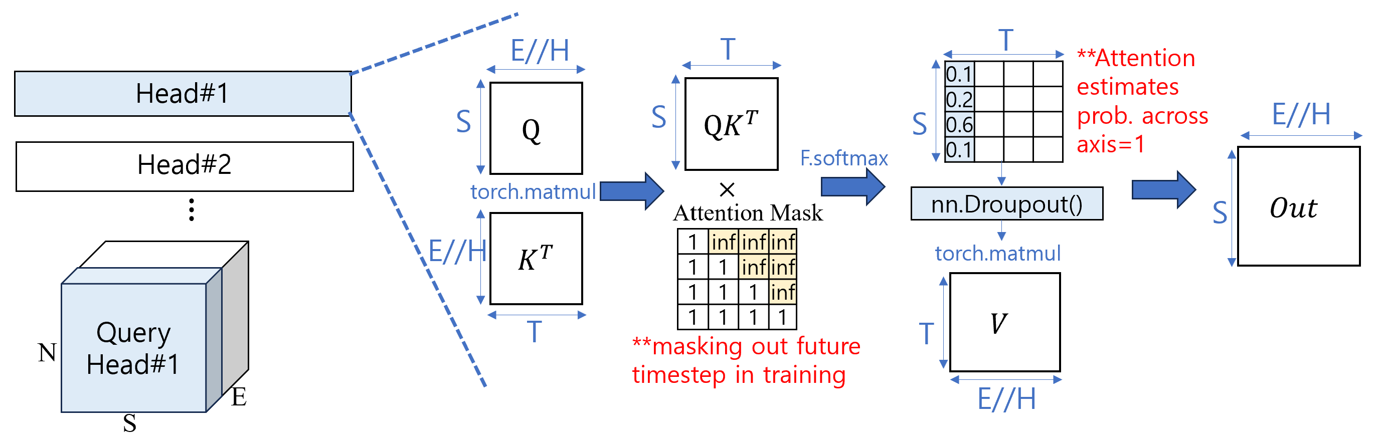
Multihead self-attention layer is composed of marix-multiplication, but with a few important distinctions. First, it is crucial to apply masking to prevent a token from looking ahead future tokens. For the illustartion above, a mask with the first row [1, inf, inf, inf] ensures that the first token can only refer to itself, not to any future tokens. Second, the target token is reference point for caculating attention scores. In the blue-highlighted box above, the first target token attends to the source tokens with weights [0.1,0.2,0.6,0.1], indicating that the third source token has the strongest influence.
class MultiHeadAttention(nn.Module):
    ....

    def forward(self, query, key, value, attn_mask=None):
        ....
############################################################################
        # TODO: Implement multiheaded attention using the equations given in       #
        # Transformer_Captioning.ipynb.                                            #
        # A few hints:                                                             #
        #  1) You'll want to split your shape from (N, T, E) into (N, T, H, E/H),  #
        #     where H is the number of heads.                                      #
        #  2) The function torch.matmul allows you to do a batched matrix multiply.#
        #     For example, you can do (N, H, T, E/H) by (N, H, E/H, T) to yield a  #
        #     shape (N, H, T, T). For more examples, see                           #
        #     https://pytorch.org/docs/stable/generated/torch.matmul.html          #
        #  3) For applying attn_mask, think how the scores should be modified to   #
        #     prevent a value from influencing output. Specifically, the PyTorch   #
        #     function masked_fill may come in handy.                              #
        ############################################################################
        H = self.n_head
        HD = self.head_dim
        query   = self.query(query).reshape(N, S, H, HD).permute(2,0,1,3)      # [H,N,S,E//H]
        key     = self.key(key).reshape(N, T, H, HD).permute(2,0,1,3)          # [H,N,T,E//H]
        value   = self.value(value).reshape(N, T, H, HD).permute(2,0,1,3)      # [H,N,T,E//H]
        similarity = torch.matmul(query, key.transpose(-2,-1))/math.sqrt(HD)   # [H,N,S,T]

        if attn_mask is not None:
            similarity = similarity.masked_fill(attn_mask == 0, float('-inf'))

        attention = F.softmax(similarity, dim=-1)
        attention = self.attn_drop(attention)

        output = torch.matmul(attention, value)     #[H,N,S,E//H]
        output = output.permute(1,2,0,3)            #[N,S,H,E//H]
        output = output.reshape(N, S, E) # (N, S, E)

        output = self.proj(output)
        ############################################################################
        #                             END OF YOUR CODE                             #
        ############################################################################
        return output
Q2: vectorized SimCLR loss
Recall the loss of pisitive pair i, j with batch N :

It’s often easier to decouple the numerator and denominator when computing InfoNCE loss. The numerator is straightforward—typically involving the cosine similarity between a positive pair—so we can safely skip detailing it here. The denominator, however, requires more care: it involves computing similarities across all pairs and masking out.
def sim_positive_pairs(out_left, out_right):
    """Normalized dot product between positive pairs.

    Inputs:
    - out_left: NxD tensor; output of the projection head g(), left branch in SimCLR model.
    - out_right: NxD tensor; output of the projection head g(), right branch in SimCLR model.
    Each row is a z-vector for an augmented sample in the batch.
    The same row in out_left and out_right form a positive pair.

    Returns:
    - A Nx1 tensor; each row k is the normalized dot product between out_left[k] and out_right[k].
    """
    pos_pairs = None

    ##############################################################################
    # TODO: Start of your code.                                                  #
    #                                                                            #
    # HINT: torch.linalg.norm might be helpful.                                  #
    ##############################################################################
    dot_map = torch.mul(out_left, out_right).sum(dim=1, keepdim=True)

    norm_left = torch.linalg.norm(out_left, dim=1, keepdim=True)
    norm_right = torch.linalg.norm(out_right, dim=1, keepdim=True)

    norm_map = torch.mul(norm_left, norm_right)

    pos_pairs = dot_map/norm_map
    ##############################################################################
    #                               END OF YOUR CODE                             #
    ##############################################################################
    return pos_pairs
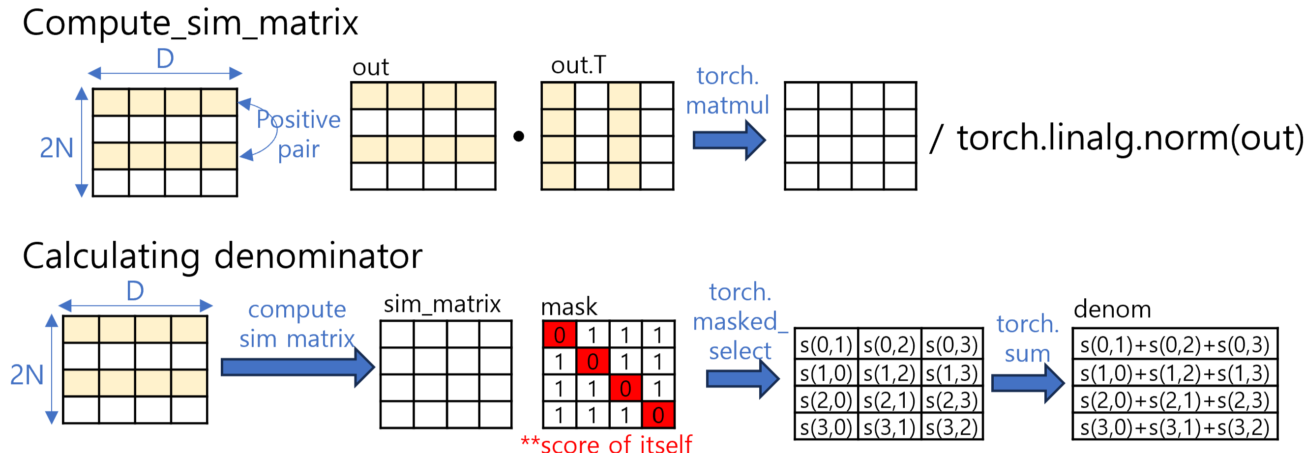
The yellow box indicates one of positive pair. In vectorized form, cosine similarity can be efficiently computed using simple matrix multiplication via compute_sim_matrix function in assignment code. However, don’t forget to mask-out in denominator for InfoNCE which exclude score of itself.
Refer to the complete contrastive_loss.py() code.
Q3: DDPM(Denoising Diffusion Probabilistic Models)
q_sample()
The main novelty of paper is to skip forward pass and directly compute from . Just implement the function paper said as below

p_loss()
compute weighte MSE loss. Note that the \epsilon-target of what model should predicts-can be noise and x_start.

p_sample()
predict noise and directly compute x_start (i.e, original image) by manipulating the paper conclusion of forward pass (i.e, q_sample()).

Frequently Asked Questions
Q1. How do you compute L2 distances between test and training matrices in KNN without explicit loops?
Expand the squared Euclidean distance ||x - y||^2 = ||x||^2 + ||y||^2 - 2 x·y^T. Compute row-wise squared norms for both X_test and X_train using np.power(X, 2).sum(axis=1), broadcast-add them, and subtract 2 * X_test.dot(X_train.T) before taking the element-wise square root.
Q2. Why does im2col speed up convolutional neural network forward and backward passes?
Although im2col duplicates overlapping receptive fields in memory, it converts sliding-window spatial convolutions into a single dense general matrix multiplication (GEMM), allowing BLAS/GPU tensor cores to execute the layer with high arithmetic intensity.